Documentation under construction. Stay tune for updates.
CBE Rad Tool
The CBE Rad Tool is an interactive web-based design tool for the early design of high thermal mass radiant systems. The primary aim of this design tool is to provide an interface for estimating the performance of high thermal mass radiant systems under steady-state conditions (for both heating and cooling) and transient conditions (on the cooling design day). High thermal mass radiant systems have a slow response time to control changes because it has to heat or cool a substantial amount of thermal mass (e.g. building's structural slab) before any noticeable effect in the thermal environment of the spaces. It has been shown that it can take over two hours for embedded surface radiant systems (ESS) and over nine hours for thermally activated building radiant systems (TABS) to change the surface temperature to a new setpoint Ning et al. (2017). Thus, it is important to use transient tools, such as the CBE Rad Tool, that considers high thermal mass radiant systems' start time and duration of operation to properly calculate the space and hydronic plant heat extraction rates. CBE Rad Tool allows designers to consider the impact of innovative control strategies such as nighttime cooling plant operations. In the sections below, this guide goes through the methods and assumptions used to develop it. The first section of the guide references the steady-state calculations while the second section references the transient calculations. There is also a third section that describes how you can request a custom radiant zone for your own analysis.
Steady-State Analysis
The steady-state analysis provides results for ESS and TABS hydronic radiant systems in cooling and heating mode. By definition, a steady-state process does not change in time. Therefore in this method of analysis, the space heat extraction rate is equal to the hydronic plant extraction rate. As a consequence, a steady-state method cannot be used to analyze the thermal inertia of the space and radiant system. Please refer to the transient method of the CBE Rad Tool to study the effect of thermal inertia. The thermal inertia of the system will have significant effects on the peak hydronic plant capacity as the start time and operation duration is changed. In the steady-state method, the tool calculates a characteristic curve that shows the relationship between the heat flux and fluid differential temperature in the tubes. The characteristic curve, or the equivalent heat transmission coefficient, depends on the radiant system construction type and other design parameters. The following section describes the input parameters to the steady-state method followed by a description of the outputs. Figure `1` shows a schematic of a thermal zone in plan view. This figure helps visualize some of the input parameters described below.
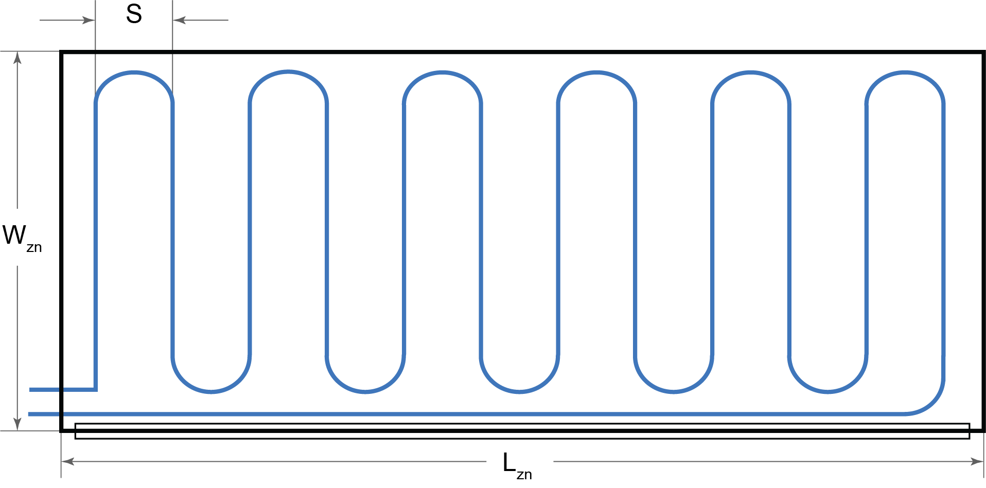
Figure `1`: Schematic of single thermal zone in plan view.
Steady-State Tool Inputs
Zone Length `(L_{zn})`
The zone length is the measurement of the zone that is collinear to the exterior wall as shown in Figure `1`. The zone length measurement is also parallel to the pipe spacing `(S)` measurement of the radiant water loop.
Zone Width `(W_{zn})`
The zone width is the measurement of the zone taken from the edge of the exterior wall into the zone as shown in Figure `1`. The zone width measurement is also perpendicular to the pipe spacing `(S)`.
Pipe Spacing `(S)`
The pipe spacing is the on-center distance between the water pipes of the radiant system. The pipe spacing in the thermal radiant zone is an important driver for the total heat flux capacity of the radiant system. The default used in the tool is 0.1520 m (6 in).
Maximum Loop Length
The maximum continuous length of one loop, or circuit, that extends from the supply manifold to the return manifold. The maximum loop length along with the pipe diameter, pipe spacing, the working fluid used in the pipe, fluid flow rate, and pressure drop requirements determine the number of loops in the user defined area of the thermal radiant zone. Note that the maximum loop length may be regulated by your local building codes. The default used in the tool is 114 m (375 ft).
Maximum Pressure Drop per Loop
The maximum pressure loss, or head loss, due to friction that is allowed in each loop of the radiant system. The default used in the tool is 10 ft of head (30 kPa).
Pipe Depth
The measurement taken from the top of the active surface (floor or ceiling) into the center of the radiant layer. The default in the tool is 0.1016 m (4 in).
Radiant Layer Thermal Conductivity
The thermal conductivity of the radiant layer where the pipes of the radiant system are embedded. For the ESS radiant system, the radiant layer is the layer that comes after the insulation layer. In the case of TABS, the radiant layer corresponds to the whole structural slab. The default in the tool is 2.1 `\frac{W}{m\cdotK}` `(14.6 \frac{Btu \cdot \i\n}{h\cdot ft^{2}\cdot ^\circF})`.
Surface Covering Thermal Resistance
The thermal resistance applied to the user selected active surface. The surface covering thermal resistance is the last layer of the radiant system construction. The default in the tool is 0.044 `\frac{W}{m^2 \cdotK}` `(0.25 \frac{h\cdot ft^{2}\cdot ^\circF}{Btu \cdot \i\n})`.
Total Slab Thickness
The thickness of the structural slab. This parameter is only used for the TABS radiant system. The default in the tool is 0.2032 m (8 in).
Supply Fluid Temperature
The temperature of the fluid at the supply manifold flowing to each of the loops, or circuits. The supply fluid temperature in the loops is an important driver for the total heat flux capacity of the radiant system. The default in the tool is `59 ^\circ F` `(15 ^\circ C)`.
Delta Temperature Between Supply and Return
The design temperature difference between the supply and return manifolds. The delta temperature between the supply and return manifold is an important parameter in calculating the fluid flow rate through the pipes. The default in the tool is `5 ^\circ F` `(2.8 ^\circ C)`.
Design Indoor Operative Temperature
The design operative temperature in the radiant thermal zone. The operative temperature is defined as a uniform temperature of an imaginary black enclosure in which an occupant would exchange the same amount of heat by radiation plus convection as in the actual nonuniform environment.
Design Dew Point Temperature
The design dew point temperature in the thermal radiant zone. The tool compares the design dew point temperature with the calculated active surface temperature to display warnings through text and visualization about the condensation risks in the zone. The default in the tool is `58 ^\circ F` `(14.4 ^\circ C)`
Steady-State Tool Outputs
Surface Temperature `(T_{surface})`
The mean steady-state surface temperature for the radiant system is based on the research by Jin et al. (2010). The surface temperature is calculated using Equation `1`. $$ T_{sf;u,l} = \frac{h_{tlt}T_{op}(1+(K_{u,l}D_{p})/\lambda_{l})+K_{u,l}T_{w}}{h_{tlt}(1+(K_{u,l}D_{p})/\lambda_{l})+K_{u,l}}\tag{1} $$ where `h_{t\l\t}` is the total heat transfer coefficient of the active surface, `T_{op}` is operative temperature of the zone, `K_{u,l}` is the heat conduction coefficient of the layer that is upper `(u)` or lower `(l)` to the pipe, depending on the location of the active surface, i.e ceiling or floor surface, `D_{p}` is the external pipe diameter, `\lambda_{l}` is the thermal conductivity of the pipe layer, and `T_{w}` is the fluid temperature in the pipe. The surface temperature, `T_{s\f}`, can be calculated for the active surface upper `(u)` or lower `(l)` to the pipe layer. The thermal conductivity of the pipe layer, `\lambda_{l}`, is calculated through the correlation found in Equation `2`. This thermal conductivity depends on the thermal conductivity of the material of the pipe `(\lambda_{p})`, the thermal conductivity of the material in which the pipes are embedded in `(\lambda_{m})`, and the area ratio `(A)` between the lower layer and pipe as calculated in Equation `3`. $$ \lambda_{l} = 8.545\ln(2.0335 + \lambda_{p})(1.1596+\lambda_{m})(1.3219+A)^{-1.4264} ~~~for~~~\lambda_{p}\lt2~W/m\cdot K\tag{2a} $$ $$ \lambda_{l} = -0.031+23.8723(0.2844+\lambda_{m})(-0.9502+A)^{-1.5753} ~~~for~~~\lambda_{p}\geq~2~W/m\cdot K\tag{2b} $$ $$ A = \frac{4SD_{p}}{\pi D^2_{p}}\tag{3} $$ where `S` is the pipe spacing length.
Fluid Differential Temperature `(\Delta\theta)`
The total surface heat flux of the active surface is proportional to the fluid differential temperature `(\Delta\theta)` as calculated in Equation `4`. $$ \Delta\theta = \frac{T_{s} - T_{r}}{\ln(\frac{T_{s} - T_{op} }{T_{r} - T_{op}})}\tag{4} $$ where `T_{s}` is the supply water temperature and `T_{r}` is the return water temperature of the radiant system water loop. `T_{op}` is the design operative temperature of the zone.
Equivalent heat transmission coefficient `(K_{H})`
The equivalent heat transmission coefficient `(K_{H})`, or the gradient of the characteristic, gives the relationship between the surface heat flux `(q_{s\f})` of the radiant system and fluid differential temperature `(\Delta\theta)`. `K_{H}` depends on radiant system type and application e.g. heating or cooling (ISO 2012).
Total Surface Heat Flux `(q_{s\f})`
The surface heat flux is calculated for the user define active surface and calculated using Equation `5`. $$ q_{sf} = K_{H}\Delta\theta\tag{5} $$
Hydronic Cooling Rate `(Q)`
The hydronic cooling rate `(Q)` is the rate at which heat is extracted by the hydronic loop of the radiant system. Since this analysis is performed with steady-state assumptions, `Q` is calculated with Equation `6`. $$ Q = q_{sf}L_{zn}W_{zn}\tag{6} $$ where `q_{s\f}` is calculated in Equation `5`, `L_{zn}` is the zone length, and `W_{zn}` is the zone width.
Total Design Fluid Flow Rate `(\dot{V}_{t\l\t})`
The total design fluid flow rate `(\dot{V}_{t\l\t})` is the total volumetric fluid flow rate for the radiant system of the whole zone. `\dot{V}_{t\l\t}` is determined on the hydronic cooling rate `(Q)` and calculated with Equation `7`. $$ \dot{V}_{tlt} = \frac{Q}{c_{p}\rho\Delta{T}}\tag{7} $$ where `c_{p}` is the specific heat of the fluid, `\rho` is the density of the fluid, and `\DeltaT` is the average temperature difference between the supply and return fluid temperature of the radiant system loops.
Design Fluid Flow Rate per Loop `(\dot{V}_{l\o\op})`
The design fluid flow rate per loop `(\dot{V}_{l\o\op})` is the total design fluid flow rate divided by the actual number loops calculated for the user define zone. The actual number of loops takes into account user defined constraints like pressure drop in pipe limit and maximum loop length. The actual number of loops is further described below.
Design Fluid Velocity in Pipe `(v)`
The design fluid velocity in the pipe `(v)` is calculated by the continuity equation shown in Equation `8`. The fluid velocity in the pipe is assumed to be a mean velocity throughout the cross section of the pipe. $$ v = \frac{4V_{tlt}}{\pi D_{i}^{2}}\tag{8} $$
Pressure Drop per Loop `(dp_{l\o\op})`
The pressure drop per loop `(dp_{l\o\op})` is calculated using the Darcy-Weisbach equation and the Swamee-Jain friction factor and shown in Equation `9`. $$ dp_{loop} = f_{d}\frac{\rho l_{act}v^{2}}{2D_{i}}\tag{9} $$ where `f_{d}` is the friction factor, `\rho` is the density of the fluid in the pipe, `l_{act}` is the length of the radiant system loop, `v` is the mean velocity in the pipe as calculated in Equation `8`, and `D_{i}` is the internal diameter of the pipe.
Actual Number of Loops `(l_{\n\um})`
The number of loops is calculated by first estimating the total pipe length `(l_{\p\ipe,t\l\t})` needed in the zone. This estimation is performed with Equation `10` and it assumes an average 10% leader length for connecting the water loops back to the radiant manifold. $$ l_{pipe,tlt} = \frac{L_{zn}W_{zn}}{S} + 2L_{zn}\tag{10} $$ where `L_{zn}` is the zone length, `W_{zn}` is the zone width, and `S` is the pipe spacing. An initial number of loops is determined by dividing by the maximum loop length defined by the user. If the initial number of loops is a fractional number, then it is rounded up to the nearest whole loop. Next, the pressure drop in each loop is calculated using Equation `9`. If the pressure drop threshold limit `dp_{max}` defined by the user is reached, then an extra loop is added to the design and the pressure drop calculation is repeated. The calculation is repeated until the pressure drop per loop is less than `dp_{max}`. After this iteration, the actual number of loop `(l_{\n\um})` is obtained.
Actual Loop Length `(l_{act})`
The actual loop length is calculated using Equation `11`. The actual length does not only depend on the zone dimensions and radiant system pipe spacing but also on the user defined constraints: pressure drop threshold limit and the maximum loop length. These constraints will have affect the actual number of loops `(l_{\n\um})` in the radiant system design. $$ l_{act} = \frac{l_{pipe,tlt}}{l_{num}}\tag{11} $$
Actual External Pipe Diameter `(D_{o})`
The user can select different pipe sizes based on nominal pipe sizes. The nominal size does not refer to an actual dimension on the pipe itself. Instead, the nominal size is just an pipe identifier where the actual dimensions, i.e. external pipe diameter, pipe wall thickness, and/or internal pipe diameter are set by national or international pipe specification standards. ASTM F876 is used in this tool to determine the actual external diameter pipe ASTM (2017).
Actual Internal Pipe Diameter `(D_{i})`
The user can select different pipe sizes based on nominal pipe sizes. The nominal size does not refer to an actual dimension on the pipe itself. Instead, the nominal size is just an pipe identifier where the actual dimensions, i.e. external pipe diameter, pipe wall thickness, and/or internal pipe diameter are set by national or international pipe specification standards. ASTM F876 is used in this tool to calculate the actual internal diameter of the pipe `(D_{i})` ASTM (2017). The standard lists the minimum wall thickness of the nominal pipe and its tolerance. Thus, half the tolerance of the pipe is added to the minimum wall thickness to obtain `D_{i}`.
Transient Analysis
A limitation of the steady-state analysis of the CBE Rad Tool is that calculations are performed under steady-state condition with a constant zone dry-bulb temperature. Steady-state assumptions are not appropriate for the design of high thermal mass radiant systems where the temperature per hour change of the active surface(s) temperature is low after a control input (change in supply water flow rate or temperature) affecting the real-time control of surface heat flux (space cooling rate) of the system. Therefore, it is often necessary to use detailed dynamic simulation tools to properly calculate the space cooling load and size the hydronic plant for these types of radiant systems. However, detailed simulation tools are complicated and time-consuming. The transient analysis of the CBE Rad Tool is easy-to-use, interactive, and web-based design tool that allows users to input values for typical design and control parameters, such as time and duration of operation for the cooling plant. The tool is especially unique because it allows designers to consider the impact of innovative control strategies such as nighttime cooling plant operation.
The transient analysis is based on pre-simulated cases on a summer cooling design day using EnergyPlus as the dynamic simulation engine. The sections below explain the available design parameters and levels for user selection, and the assumptions we used to build the single zone EnergyPlus model. This single radiant zone represents a perimeter middle floor of a large office building as shown in Figure `2` i.e. the floor and ceiling surfaces are thermally interconnected. That is, the heat flux of the top of the ceiling surface and the bottom of the floor surface is the same. We then extract time series values that include surface heat flux and hydronic system cooling rate from the EnergyPlus simulation for visualization to the user.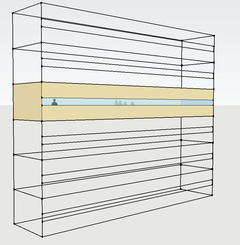
Figure `2`: Schematic of EnergyPlus model representing a perimeter middle floor radiant zone of a large office building i.e. the floor and ceiling surfaces are thermally interconnected. That is, the heat flux of the top of the ceiling surface and the bottom of the floor surface is the same.
EnergyPlus Model Description
Geometry
The geometry for the single radiant thermal zone stays constant for all simulation cases. The length `(L_{zn})` of the zone is 75 ft (22.7 m), 15 ft (4.57 m) wide `(W_{zn})`, and 10 ft (3.05 m) high `(H_{zn})`. The total floor surface area of the zone is `1125 ft^2` `(103.7 m^2)` and total volume is `18750 ft^3` `(316 m^3)` The direction of the dimensions with respect to the radiant loop is shown in Figure `1`. We used a single ribbon window with no shading system to define fenestration of the thermal zone that spans most of the length of the zone. Please note that the height of the window will change depending on window-to-wall `(WWR)` selected.
Construction Layers
We assumed one exterior wall in the radiant thermal zone. We defined the exterior wall as a medium thermal mass wall with three layers. The outside layer is normal weight concrete with thickness, thermal conductivity, specific heat, and density of `3.9 \i\n` `(100 mm)`, `8.32 \frac{Btu\cdot \i\n}{h \cdot ft^{2} \cdot ^\circ F}` `(1.2 \frac{W}{m\cdotK})`, `0.191 \frac{Btu}{lb \cdot ^\circ F}` `(0.8 \frac{kJ}{kg\cdotK})`, `140 \frac{lb}{ft^{3}}` `(2240 \frac{kg}{m^{3}})`, respectively. The middle layer is an insulation layer with thickness, thermal conductivity, specific heat, and density of `2.3 \i\n` `(59 mm)`, `0.21 \frac{Btu\cdot \i\n}{h \cdot ft^{2} \cdot ^\circ F}` `(0.03 \frac{W}{m\cdotK})`, `0.358 \frac{Btu}{lb \cdot ^\circ F}` `(1.5 \frac{kJ}{kg\cdotK})`, `0.94 \frac{lb}{ft^{3}}` `(15 \frac{kg}{m^{3}})`, respectively. The inside layer is plasterboard with thickness, thermal conductivity, specific heat, and density of `0.5 \i\n` `(13 mm)`, `1.11 \frac{Btu\cdot \i\n}{h \cdot ft^{2} \cdot ^\circ F}` `(0.16 \frac{W}{m\cdotK})`, `0.26 \frac{Btu}{lb \cdot ^\circ F}` `(1.1 \frac{kJ}{kg\cdotK})`, `50 \frac{lb}{ft^{3}}` `(800 \frac{kg}{m^{3}})`, respectively. The total U-value of the wall is `0.0616 \frac{Btu}{h \cdot ft^{2} \cdot ^\circ F}` `(0.35 \frac{W}{m^{2}\cdotK})`. We define the three other vertical walls with an adiabatic boundary condition. The ceiling and floor are thermally interconnected to represent a middle floor zone.
The solar heat gain coefficient (SHGC) and U-value for the window stays constant for all simulation cases. We defined the SHGC as 0.25 and U-value of `0.352 \frac{Btu}{h \cdot ft^{2} \cdot ^\circ F}` `(2.0 \frac{W}{m^{2} \cdot K})` which are the limits in Title 24-2013. The area of the window can be adjusted through the window-to-wall ratio as described below.
Radiant System
We maintained the ceiling/floor slab thickness constant for all simulation cases since we found that there were not significant impact of the cooling rates at the cooling design day as the slab thickness varied. The thickness of the slab is `8 \i\n` `(203.3 mm)` and made of normal weight concrete. We define the concrete with thermal conductivity, specific heat, and density of `12.5 \frac{Btu\cdot \i\n}{h \cdot ft^{2} \cdot ^\circ F}` `(1.8 \frac{W}{m\cdotK})`, `0.215 \frac{Btu}{lb \cdot ^\circ F}` `(0.9 \frac{kJ}{kg\cdotK})`, `140 \frac{lb}{ft^{3}}` `(2240 \frac{kg}{m^{3}})`, respectively. The pipe depth is also maintained constant throughout all simulation cases at `2 \i\n` `(0.051 m)` measured from the user selected active surface to the outer diameter of the pipe. The user has control over several design parameters listed below including radiant system start time and operation duration. The water flow rate is calculated using steady-state methods prior to simulation of the model and the calculated value maintained constant during the simulation at the cooling design day. Please note that the radiant system will operate at full capacity during the user selected operation duration. There is no controls to maintain the zone at a specified temperature setpoint or range. As the radiant system operation is increased, the operative temperature in the zone will decrease and vice versa. In annual simulations where the design condition. In the case of an annual simulation, of radiant control are needed to maximize thermal comfort in the space. You can refer to the CBE radiant system sequences of operation with a version of the sequences demonstrated and analyzed in Raftery et al. (2017).
Ventilation System and Infiltration
We defined the ventilation system with dual setpoints at 59 and 70°F (15 and 21°C). The ventilation airflow is oversized by 30% over Title-24 2013 which is common practice for DOAS systems to receive credits under rating systems such as LEED (Paliaga et al. 2017). The peak infiltration is `(0.537 \frac{l}{s\cdotm_{2}})` of exterior surface, or 0.64 air changes per hour. Infiltration is at 100% when the heating ventilation and air conditioning system (HVAC) is OFF. When the HVAC is ON, we reduce it to 25% of the peak infiltration.
Weather Data for Cooling Design Day
We use the same summer cooling design day for all simulation cases since it is computationally expensive to pre-simulate additional cooling design days. In addition, we expect a high performance envelope for buildings with radiant systems where the outside temperatures have small effects on the energy conducted through the opaque walls. The solar heat gains has a significantly greater impact on the performance of the radiant system. The solar heat gains can be varies in this tool by using the zone orientation and/or the window-to-wall ratio described above. The cooling design day is defined for a site latitude of 40°N on July 21 with a maximum outdoor dry-bulb temperature of 95°F (35°C) and daily temperature range of 21°F (11.7°C). We obtained these cooling design day parameters from ASHRAE studies on the cooling load (Rudoy and Duran (1975) Spitler, McQuiston, Lindsey (1993)).
Internal Gain Schedules
We defined the internal gain schedules in all simulation cases with values found in the US DOE large office prototype building model US DOE (2013), which is defined for a typical building compliant to ASHRAE 90.1-2013 standard. These schedules include lighting, plug load, occupancy, and infiltration. Figure `3` shows the schedules for lighting, plug load, and occupancy.
The ventilation air system is set to operate from 7:00 to 18:00 on the cooling design day within the temperature setpoints defined in Ventilation System and Infiltration section. The infiltration schedule is set to 0.25 from 7:00 to 18:00 and 1 for all other hours.
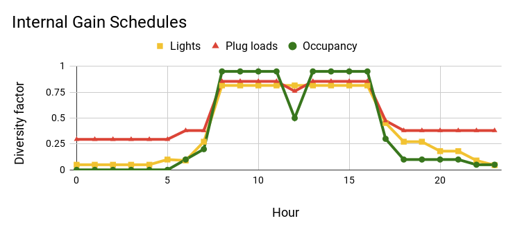
Figure `3`: Lighting, plug load, and occupancy schedules for all simulation cases in the CBE Rad Tool. We obtained the values from the DOE large office prototype building model US DOE (2013).
Transient Tool Inputs
The following design parameters are parameters that can be selected by the user through drop down menus.
Zone Orientation
This is the orientation of the exterior wall of the single thermal zone. Note that there is only one exterior wall as described above and the other three surfaces have an adiabatic boundary condition. The available levels for this parameter are South, West, North, and East.
Window-to-Wall Ratio (WWR)
The window-to-wall ratio (WWR) is a ratio that defines the amount of glazing on the exterior wall. This measurement is the fraction of glazing to the total exterior wall area of the thermal zone. Since the geometry is constant throughout all simulation cases, the area of the glazing can be determine by multiplying the select WWR percentage by `750 ft^{2}` `(69.2 m^{2})`. The WWR is an important parameter to vary the solar heat gain entering the thermal zone. The available levels for this parameter are 20% and 60%.
Radiant Operation Start Time
The radiant operation start time defines when the radiant system starts to operate during a 24-hour period. The available levels for this parameter are hours between 0:00 and 23:00 in 2-hour increments.
Radiant Operation Duration
The radiant operation duration define the total number of hours that the radiant system operates within a 24-hour period. The available levels for this parameter are hours between 8 and 24 in 2-hour increments.
Supply Water Temperature
The water temperature at the supply manifold flowing to each of the loops, or circuits. The supply water temperature in the loops is an important driver for the total heat flux capacity of the radiant system. The available levels for this parameter are supply water temperatures 55, 57, and 61 °F (12.78, 13.89, and 16.11 °C).
Design Water Temperature Difference
The design temperature difference between the supply and return manifolds. The delta temperature between the supply and return manifold is an important parameter in calculating the fluid flow rate through the pipes. The available levels for this parameter are delta temperatures 3, 5, and 8°F (1.7, 2.8, and 4.4 °C).
Pipe Spacing `(S)`
The pipe spacing is the on-center distance between the water pipes of the radiant system. The pipe spacing in the thermal radiant zone is an important driver for the total heat flux capacity of the radiant system. The available levels for this parameter are 2 in (0.1524 m) and 12 in (0.3048 m).
Internal Pipe Diameter `(D_{i})`
This parameter defines the internal pipe diameter of the radiant system. It is used in conjunction with other parameters to define the water flow rate through the system. The available levels for this parameter are the pipe internal diameters 0.35, 0.475, and 0.574 in (8.9, 12.1, and 14.6 mm).
Maximum Loop Length
The maximum continuous length of one loop, or circuit, that extends from the supply manifold to the return manifold. The maximum loop length along with the pipe diameter, pipe spacing, the working fluid used in the pipe, fluid flow rate, and the pressure drop requirements determine the number of loops in the thermal radiant zone. Note that the maximum loop length may be regulated by your local building codes. The available levels for this parameter are 300, 350, and 400 ft (91.4, 106.7, and 121.9 m).
Night Time Plug Load Baseload Fraction
The night time plug load baseload fraction directly overrides the schedule values for the plug load equipment during unoccupied hours i.e. 0:00 to 8:00 and 18:00 to 23:00. The available levels for this parameter are 10, 20, and 30%.
Heat Gain Rate
The heat gain rate defines the design heat gain rate for lighting, plug loads, and occupancy. In the tool, we use three categories where the three heat gain rates are modified at the same time as opposed to modifying them individually. The available levels for this parameter are three categories: low, medium, and high and the values are shown in Table `1`.
Table `1`: The design internal heat gain rates for lights, plug load, and occupancy at each category that users can select.
| Category | Lights `{Btu}/{h \cdot ft^{2}}` `(W/m^{2})` | Plug Loads`{Btu}/{h \cdot ft^{2}}` `(W/m^{2})` | Occupancy `{ft^{2}}/{person}` `(m^{2}/{person})` |
|---|---|---|---|
| Low | 1.6 (5) | 6.3 (20) | 54 (5) |
| Medium | 2.4 (7.5) | 3.4 (10.8) | 85 (7.9) |
| High | 2.7 (8.6) | 5.7 (18) | 65 (6) |
Active Surface
The user can select the ceiling or the floor as the active surface. The radiant system pipes are the closest this selected surface. That is, the pipe depth is always 2 in (0.0508 m) from the selected active surface. The active surface will have the greatest surface heat flux than the other non-selected surface.
Transient Tool Outputs
We directly extracted the listed outputs below from the EnergyPlus simulation results of the model described above. These results include 24-hour profile displayed in the plots while other are one metric values listed in tables.Surface Heat Flux
The surface heat flux is the flow of energy per unit of time for the active surface selected. In the case of TABS systems, the ceiling and the floor surface are active surfaces. Thus, the surface heat flux for both surfaces are added together to display one 24-hour profile.
Hydronic Cooling Rate `(Q_{t})`
The hydronic cooling rate `(Q_{t})` is the rate at which heat is extracted by the hydronic loop of the radiant system. In the transient analysis, the hydronic cooling rate is rarely, if ever, equal to the surface heat flux of the active surface. This is because the transient analysis takes into account the thermal inertia of the thermal mass in the room which includes the ceiling/floor slab.
Heat Gain Rate
The heat gain rate is the energy entering or being generating inside the space. This 24-hour profile includes energy from the following sources: net energy through the envelope i.e. solar radiation energy through the windows and energy conducted through the opaque walls, plug loads, and lighting. It also includes net energy entering from ventilation and infiltration.
Operative Temperature
The operative temperature is defined as a uniform temperature of an imaginary black enclosure in which an occupant would exchange the same amount of heat by radiation plus convection as in the actual nonuniform environment.
Water Flow Rate
The design water flow rate through the radiant pipes embedded in the radiant layer of the radiant system. The water flow rate is calculated prior to starting the dynamic simulation of the selected radiant zone. The water flow rate is calculated using the same method as in the steady-state analysis of the tool. That is, design parameters from the dynamic radiant zone are used to calculate the steady-state hydronic cooling rate to then calculate the water flow rate with Equation `7`.
References
ASTM, 2017. ASTM F876:2017 - Standard Specification for Crosslinked Polyethylene (PEX) Tubing.
ISO, 2012. ISO 11855:2012 - Building environment design-Design, dimensioning, installation and control of embedded radiant heating and cooling systems. International Organization for Standardization, Geneva, Switzerland.
Jin, X., Zhang, X., Luo, Y., 2010. A calculation method for the floor surface temperature in radiant floor system. Energy and Buildings 42, 1753–1758. https://doi.org/10.1016/j.enbuild.2010.05.011
Ning, B., Schiavon, S., Bauman, F.S., 2017. A novel classification scheme for design and control of radiant system based on thermal response time. Energy and Buildings 137, 38–45. https://doi.org/10.1016/j.enbuild.2016.12.013
Paliaga, G., Farahmand, F., Raftery, P., Woolley, J., 2017. TABS Radiant Cooling Design & Control in North America: Results from Expert Interviews. eScholarship. http://escholarship.org/uc/item/0w62k5pq
Raftery, P., Duarte, C., Schiavon, S., Bauman, F., 2017. A new control strategy for high thermal mass radiant systems, in: Proceedings of Building Simulation 2017. http://escholarship.org/uc/item/5tz4n92b
Rudoy, W., Duran, F., 1975. Development of an improved cooling load calculation method. ASHRAE Transactions 81, 19–69.
Spitler, J.D., McQuiston, F.C., Lindsey, K.L., 1993. The CLTD/SCL/CLF cooling load calculation method. ASHRAE Transactions 91, 183–192.